Written by Matthew R.
Introduction
In search of a combination of investments that provide the maximum return in a volatile market, private investors, traders and fund managers are faced with an asset allocation problem (Parigi and Pelizzon, 2008). The optimal strategy should be based on a model that estimates, assesses and manages uncertainty. One of the most popular approaches to asset allocation is the mean-variance portfolio optimisation based on the Modern Portfolio Theory (Markowitz, 1952, 1959).
The aim of this approach is to allocate funds in such a way that the maximum return on investment for a given level of risk would be achieved. In other words, such allocation is targeted at reducing portfolio risk. Risk in this context is defined as the possible variation of expected returns and proxied by the standard deviation of the portfolio's historic returns (Markowitz, 1952, 1959).
The goal of this paper is to construct and analyse the mean variance portfolio performance. In the first part of this paper, three portfolios are constructed from ten randomly selected stocks from the FTSE 100 Index. These include the Naïve portfolio, Minimum Variance portfolio and Tangent portfolio. Daily stock prices are used for the period from 2012 until 2016. In the second part of this paper, the performance of these portfolios and the benchmark FTSE 100 Index is evaluated using the Sharpe Ratio, the Treynor Ratio and Average Annualised Returns. After careful considerations, a recommendation to investors is provided on whether to use this approach in practice.
Portfolio Construction
Ten randomly selected stocks from the FTSE 100 have been selected. These stocks include Admiral Group (ADM); British Petroleum (BP); HSBC Holdings (HSBA); Kingfisher (KGF); Lloyds Banking Group (LLOY); Morrison Supermarkets (MRW); National Grid (NG); Rolls-Royce Holdings (RR); RSA Insurance Group (RSA) and Vodafone (VDF). The evaluation period for portfolio construction is from January 01, 2012 until December 31, 2016. The data has been collected from the London Stock Exchange (2018).
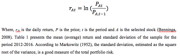
In portfolio construction, the first essential step is to calculate the return on the selected stocks. This return is earned by investors who buy the stock at the end of period t-1 and sell them at the end of period t (Benninga, 2008). Daily returns for each stock are calculated using an assumption that all returns are reinvested in the portfolio and there is no payment of dividends on these shares. Therefore, the continuously compounded return formula is used in calculations:

The historical returns on MRV and RR are negative. This means that for the period 2012-2016, these stocks were on average losing value. Expected returns on all other stocks are positive. Based on the estimated historical returns, the variance-covariance matrix has been constructed. This matrix is required to calculate the mean-variance portfolios and the Efficient Frontier. The variance-covariance matrix for the ten selected stocks is provided in Appendix.
Next, the three mentioned portfolios are constructed. The Naïve or Equally Weighted portfolio is the portfolio where capital is evenly invested in several risky assets regardless of their risks and returns. According to Tang (2004), Naive portfolios allow the investor to reduce the portfolio risk effectively without compromising the expected rate of return. In the portfolio of 10 assets, the amount of money invested in each stock is 10%. Thus, the number of shares of each asset differs depending on the share price. Some analysts argue that since stock prices change rapidly, the Naive portfolio needs a constant rebalancing to maintain an equal weight of assets (Malaj, 2011). The mean return of this portfolio is the average return of all 10 stocks for the period. The expected returns on the portfolio could also be expressed by the following formula:

However, the Naïve portfolio does not maximise returns for a given level of risk. Markowitz (1952) in his Modern Portfolio Theory suggested an alternative strategy. This approach proposes the search for a combination of assets that yields the highest return with the given standard deviation or total variance. A particular case of this optimisation is the Minimum-variance portfolio, which is the portfolio that minimises the risk of the portfolio.
The tangent portfolio in the Markowitz framework is the portfolio that provides the maximum return on investment adjusted for risk, expressed as the standard deviation, e.g. it has the highest Sharp ratio (Benninga, 2008). The Tangent Portfolio shows the best combination of risky and risk-free assets. As a proxy of daily returns of a risk-free asset, the 12 Month LIBOR rate is used in this paper (Federal Reserve Economic Data, 2018). The tangent and minimum-variance portfolios are calculated using MS Excel as proposed by Benninga (2008). Information about portfolios weights, mean returns and standard deviations is given in Table 2.

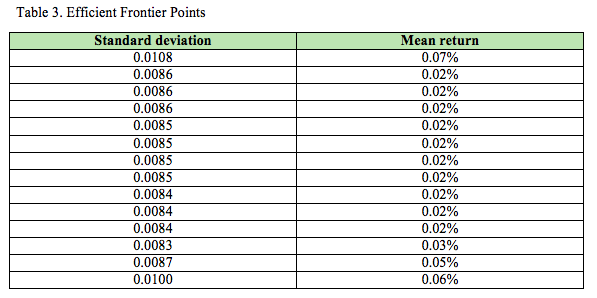
Efficient frontier is the aggregate of all possible optimal portfolios that, for each standard deviation, provide the highest expected return (Markowitz, 1952). Visually, the efficient frontier is represented by a curve with the expected return on the y-axis and standard deviation on the x-axis. The curve has a positive slope and extends from the minimum variance portfolio upwards (Malaj, 2011). To construct the Efficient Frontier, several envelope portfolios are estimated and the convex combinations of these portfolios are the basis for calculation of the efficient frontier points (Table 3).
Based on the calculations above, the efficient frontier graph is presented in Figure 1. The three constructed portfolios are shown on the graph based on their mean return and standard deviation.
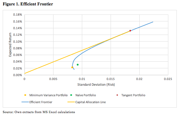
The minimum variance portfolio has the lowest risk and is located at the start of the efficient frontier. In other words, it is the extreme left portfolio on the graph. According to the Modern Portfolio Theory (Markowitz, 1952, 1959), all portfolios that have higher standard deviation or risk but lower expected returns are inefficient. The naive portfolio does not maximise the reward for a given level of risk. It could be observed from Figure 1 that the Naïve portfolio is located below the efficient frontier. Therefore, the equally weighted portfolio of 10 selected stocks is feasible, but not efficient.
The tangent portfolio lies on the intersection of the efficient frontier and Capital Allocation Line (CAL). CAL shows a combination of the risk-free asset and the risky portfolio and touches the efficient frontier at the point where the risk adjusted returns measured by the Sharpe ratio are maximised (Sharpe, 1994). Therefore, the tangent portfolio is the portfolio with the highest return-to-volatility ratio on the efficient frontier.
In order to maximise wealth, an investor can hold a market portfolio or a portfolio of risky assets with the same risk-adjusted return. Risk averse investors are ready to accept higher risk in order to get higher returns. Risk-neutral investors are indifferent between risky and riskless investments as long as they provide the same returns. Risk seeking investors prefer risky assets even if they provide lower returns. The Modern Portfolio Theory and the mean-variance approach make an assumption that all investors are risky averse. Portfolios below the efficient frontier are not optimal; thus such investments are not recommended.
Performance Analysis
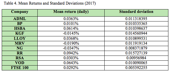
In order to evaluate the performance of the constructed portfolios, the paper analyses several performance metrics such as the Sharpe ratio and the Treynor ratio. In addition to this, the FTSE 100 Index is used as a benchmark (London Stock Exchange, 2018). Table 4 presents the mean return and standard deviation of the constituents of the constructed portfolios on an individual basis in 2017, which is the test period.
The first metric for the analysis is the Sharpe ratio. It is a commonly used benchmark that describes how well the return on investment justifies the accepted risk (Jobson and Korkie, 1981). The Sharpe ratio is calculated as the excess return on a portfolio divided by its standard deviation. A greater Sharpe ratio is desirable as it shows that an optimal portfolio would have the highest return-to-volatility relationship (Sharpe, 1994; Benninga, 2008). The Sharpe ratios for the constructed portfolios are presented in Table 5.
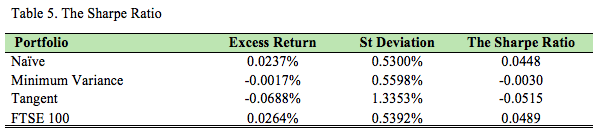
The Sharpe ratio of all mean-variance portfolios (tangent and minimum variance) is negative, which means that the returns of all these assets were lower than the risk-free rate in 2017. However, the FTSE100 has the best ratio. As stated by the Modern Portfolio Theory, systematic or market risk cannot be diversified.
The second metric is the Treynor ratio that measures the excess return adjusted for the market volatility or the systematic risk (Jobson and Korkie, 1981). According to Scholz and Wilkens (2005), the Sharpe and Treynor ratios of well-diversified portfolio are similar, because the total risk and the systematic risk for such portfolio should be similar (Billio et al., 2010). However, this rarely happens in practice due to inability to reach perfect diversification. The FTSE 100 Index is used as a basis for market volatility. The Treynor ratio is compared across the constructed portfolios in Table 6.
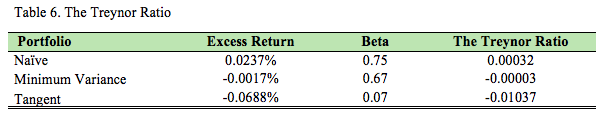
The market beta for all portfolios is less than one. Therefore, each portfolio is less volatile than the FTSE 100 Index. The Tangent portfolio has the lowest beta of 0.07 while the Naïve portfolio has the highest beta of 0.75. However, the Treynor ratios of the mean-variance portfolios are negative as the expected returns are lower than the risk-free rate. Based on the Treynor ratio, all portfolios except for the Naïve portfolio produced weak results in 2017.
The last performance metric used in this analysis is the average annualised return. For this purpose, the mean return of each portfolio is multiplied by the number of trading days in a year. The summary of the results is shown in Table 7.
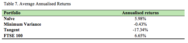
It can be noted that the Naïve portfolio shows the best annualised return of 5.98% supporting Tang’s (2004) conclusions on the superiority of this portfolio management strategy. However, the benchmark FTSE 100 Index shows even higher returns of 6.65%. The Minimum-Variance and Tangent portfolios show negative returns. These results indicate that despite its advantages, the Modern Portfolio Theory is based on historical data and is not able to provide investors with an instrument that allows them to construct the optimal portfolio in a volatile market.
Conclusion
This paper applied the Modern Portfolio Theory and constructed three portfolios based on daily market data for ten randomly selected stocks from the FTSE 100 Index. The results of the performance analysis show that the Minimum Variance and Tangent portfolios failed to provide an optimal solution to investors in a volatile environment in the post-estimation period. Despite the highest Sharpe ratio for the period 2012-2016, in 2017 the Tangent portfolio showed the worst average annualised return amounting to -17.34%. On the other hand, the Naïve portfolio provided a solid yield of 5.98% to investors.
Based on the results of the analysis, it could be stated that the mean variance approach to portfolio construction does not provide an optimal solution for investors in practice. On the other hand, there is no such tool that would allow investors to always have a perfectly balanced portfolio. Any portfolio based on historical data would be subject to similar limitations. Nevertheless, the further development of the Modern Portfolio Theory could lead to the creation of new tools, which will help investors to create more efficient portfolios.
References
Benninga, S. (2008) Financial Modelling. Cambridge: The MIT Press. pp. 239-333.
Billio M., Getmansky, M., Lo, A.W. and Pelizzon, L. (2010) Econometric Measures of Systemic Risk in Finance and Insurance sectors. MIT WP 4774-10, NBER Working Paper №16223.
Federal Reserve Economic Data (2018) 12-Month London Interbank Offered Rate, [Online] Available at: https://fred.stlouisfed.org/series/GBP12MD156N, [Accessed: January 16, 2018].
Jobson, J. and Korkie, R. (1981) Performance Hypothesis Testing with the Sharpe and Treynor Measures. Journal of Finance. 36. pp. 889–908.
London Stock Exchange (2018) FTSE 100 Index Historic Information, [Online] Available at: http://www.londonstockexchange.com/exchange/prices-and-markets/stocks/indices/summary/summary-indices.html?index=UKX, [Accessed: January 16, 2018].
Malaj, V. (2011) Modern Portfolio Theory: Identification of Optimal Portfolios and Capital Asset Pricing Model Test. CEA Journal of Economics. 6(2). pp. 53-65.
Markowitz, H. M. (1952) Portfolio Selection. The Journal of Finance. 7(1). pp. 77–91.
Markowitz, H. M. (1959) Portfolio Selection: Efficient Diversification of Investments. New York: John R. Wiley and Sons. pp. 37-80.
Parigi, B., and Pelizzon, L. (2008) Diversification and ownership concentration. Journal of Banking and Finance. 32(9). pp. 1743-1753.
Scholz, H. and Wilkens, M. (2005) An investor-specific performance measurement: A justification of Sharpe ratio and Treynor ratio. International Journal of Finance. 17(4). pp. 3671-3691.
Sharpe, W. (1994) The Sharpe Ratio. Journal of Portfolio Management. 21. pp. 49–58.
Tang, G. Y. N. (2004) How Efficient is Naïve Portfolio Diversification? An Educational Note. OMEGA: International Journal of Management Science. 32(2). pp. 155–160.
")