Written by Carl R.
The purpose of this study is to model and forecast the volatility of the FTSE 100 index returns using Generalised Autoregressive Conditional Heteroscedasticity (GARCH) models (Bollerslev, 1986; Bollerslev, 1990; Bollerslev and Engle, 1986; Engle, 1982; Engle, 2001). The GARCH model with t-distribution brings significant results in the ARCH and GARCH effects; Table 1 provides the output of the complete regression.
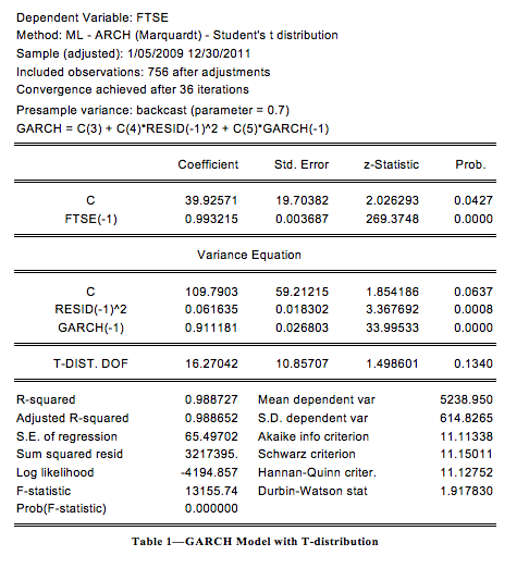
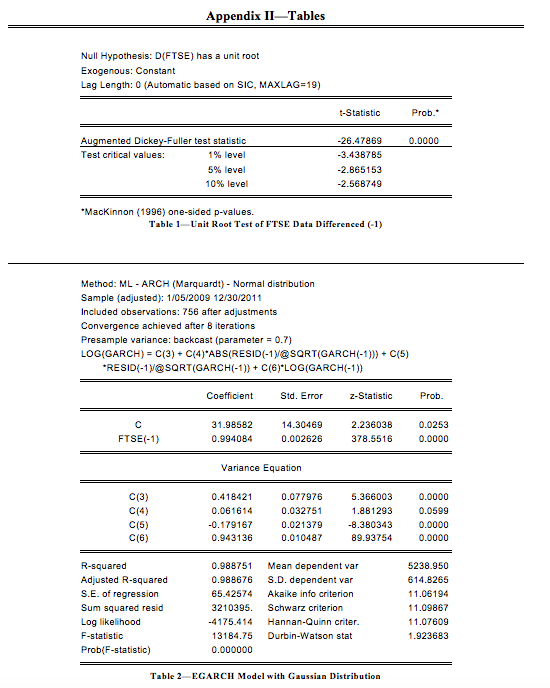
These results suggest that there is a quite strong persistence in volatility of the FTSE 100 index as the GARCH term has a coefficient above 0.9. The t-distribution model is then compared to the same GARCH model with the Gaussian distribution (Hall and Yao, 2003; Nelson, 1991; Geweke, 1986). Table 2 provides the output of the regression.
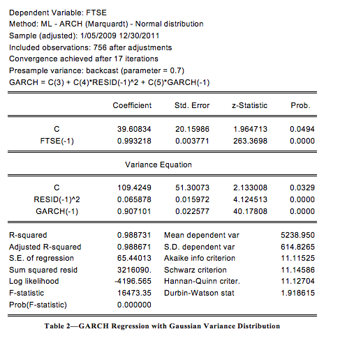
All coefficients are significant in the variance equation, and it is confirmed that there is presence of volatility persistence similar to the GARCH model with t-distribution. Also the Akaike and Schwarz criteria (Gujarati, 2003) are nearly the same suggesting that none of these models could be considered superior to the other.
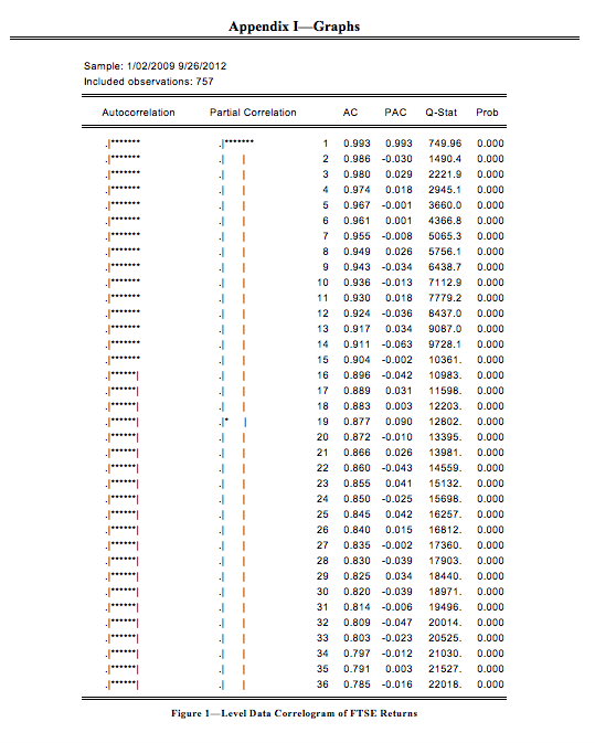
Figure 1, below, is a graph of the modeled points of the GARCH model fitted to the actual data. As expected, there is little observable difference between the modeled data and the information. The residuals indicate the volatility in the data is consistent throughout the model; however, there are three noticeable periods of higher than average volatility: the first three months of 2009, the second quarter of 2010 and the third quarter of 2011. All three periods are when the market declined.

The second part of the data will require the actual forecast of the variance during the time period, which should be cautioned because of the three aforementioned periods which had greater than normal residuals. However, the forecast of variance reduces quickly as the variance declines indicating a period of relative stability from September 2009 onward. Therefore the model should feel suitable to model the data.
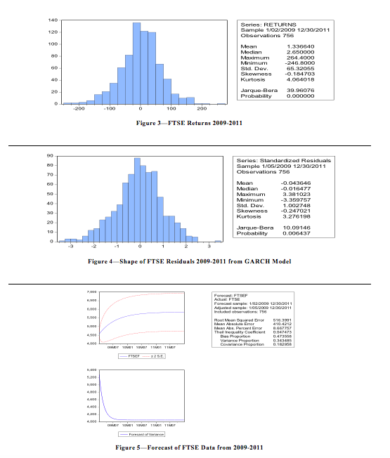
A close look at the residuals calls into question the validity of the model. One of the assumptions of the test claims the residuals should follow a normal distribution. The residuals, however, fail to do so. In fact, the kurtosis is higher than normal, the skewness is negative, and the Jarque-Bera stat p-value is near 0. The requirement for a normal distribution can be relaxed as finding a perfectly normal distribution is difficult in financial time-series (Gujarati, 2003).
The variance in the dataset still assumes the variance will increase at a decreasing rate; however, the actual data eliminates the possibility of this occurrence. The actual data varies greater than the model suggests. Mostly, the data fluctuates between periods of high and low volatility. A major reason could be the presence of autocorrelation in the level and second difference data. One reason for a larger fluctuation is that the basis period by which the data is modeled around sees a decline during the 2012 year, which is consistent with the earlier observation that a decline will encounter greater fluctuations in the volatility. A number of events happened during the year which could have influenced the lack of investor confidence in the market. Namely, the European debt crisis, austerity measures in the United Kingdom, and a slowdown in the growth of China. The forecasted data showed quite the opposite: a moderate increase in the FTSE.
| Figure 2—Forecast of Variance and Conditional Variance of FTSE 100 |
This dilemma strikes at the heart of the problem of modeling discussed earlier. One way to correct for the increased negativity is to apply the asymmetric GARCH model which adjusts for continual market decline and asymmetric response of share prices to positive and negative shocks. However, more expanded dataset should be included to take advantage of the covariance seen between the market and other variables. A model with these variables will provide a more accurate forecast (Brandt and Jones, 2006; Bera and Higgins, 1993).
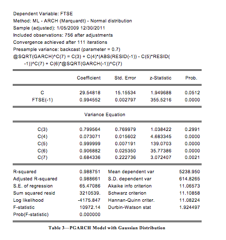
GARCH, EGARCH and PGARCH models were run in order to verify the results found above. Contrary, to what might be expected, the PGARCH and EGARCH models were in fact better fits of the data than previously assumed. The Akaike and Schwarz criterions indicated the models were superior to that of the traditional GARCH model. However, as can be observed in the table below, the difference between these models is negligible at best. Insignificant terms were found in all but the original GARCH model run with the Gaussian distribution.
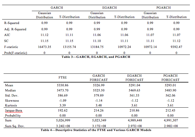
To further validate the point, forecasts were run with each model, forecasting until September 2012. Figure 3 indicates the GARCH model a superior match of the data thus far as its trend line intersect at nearly the same position as the last observation in the data.
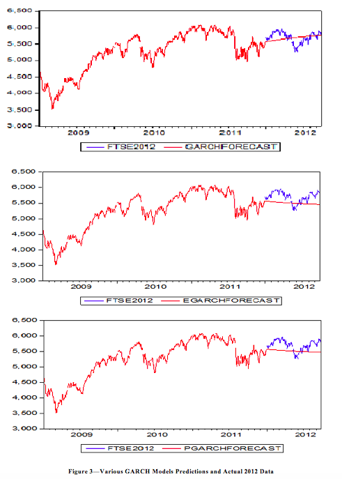
Both the EGARCH and PGARCH models were erroneous in their forecasts, even though the sums of their squared deviations were lower than that found in the GARCH. However, it is shown that the GARCH value sum of squared deviations was closer to that of the actual data.
References
Bera, A. and Higgins, M. (1993) ARCH Models: Properties, Estimation and Testing. Journal of Economic Surveys, 7 p.305-366.
Bollerslev, T. (1986) Generalized Autoregressive Conditional Heteroskedasticity. Journal of Econometrics, 31 p.307-327.
Bollerslev, T. (1990) Modeling the Coherence in Shortrun Nominal Exchange Rates: A Multivariate Generalized ARCH Approach. Review of Economics and Statistics, 72 p.498-505.
Bollerslev, T. and Engle, R. (1986) Modeling the Persistence of Conditional Variances. Econometric Reviews, 5 p.1-50.
Brandt, M. and Jones, C. (2006) Volatility Forecasting With Range-Based EGARCH Models . American Statistical Association Journal of Business & Economic Statistics , 24 (4), p.470-486 .
Engle, R. (1982) Autoregressive Conditional Heteroscedasticity with Estimates of the Variance of the United Kingdom Inflation. Econometrica, 50 (4), p.987-1007.
Engle, R. (2001) GARCH 101: The Use of ARCH/GARCH Models in Applied Econometrics. Journal of Economic Perspectives, 15 (4), p.157–168.
Geweke, J. (1986) Modeling the Persistence of Conditional Variances: A Comment. Econometric Review, 5 p.57-61.
Gujarati, D. (2003) Basic Econometrics, New York: McGraw Hill Professional.
Hall, P. and Yao, Q. (2003) Inference in ARCH and GARCH Models with Heavy-tailed Errors. Econometrica, 71 (1), p.285-317.
Nelson, D. (1991) Conditional Heteroskedasticity in Asset Returns: A New Approach. Econometrica, 59 p.347-370.
Appendices

")