Written by Anton V.
Executive Summary
This study focuses on the modelling of oil price behaviour during the period 2012-2017. The Geometric Brownian Motion (GBM) and Mean-Reversion Jump Diffusion (MRJD) models are used for this purpose. Based on the results, no substantial difference has been found between the simulated prices due to the slow speed of mean reversion and low jump intensity estimated for the MRJD model. This can be explained by the potential existence of two distinct regimes of the oil price behaviour associated with the 2014 drop in oil prices. The MRJD model reproduces volatility smiles for the arithmetic average options showing that lower volatility is associated with the at-the-money options.
1. Introduction
Market volatility has received great attention in academic literature. It is crucial for understanding the behaviour of prices and spillover effects. Furthermore, it is used to price financial assets such as exotic derivatives. Numerous techniques have been proposed to model volatility. These techniques account for the observed characteristics of financial series such as mean-reversion and large jumps. It could be useful to explore commonly employed models with regards to commodity markets. This may be especially important in the context of the 2014 drop in oil prices.
The aim of the present study is to examine how stochastic models can be used to model oil prices. This is achieved by following several steps. Firstly, two types of models are calibrated based on historical data on oil prices during the period 2012-2017. Secondly, the characteristics of simulated prices are compared between the models. Finally, the simulated prices are used to price arithmetic average options and to estimate the implied volatility of the options.
2. Background
The Black-Scholes model (Black and Scholes, 1973) has been often used as a basis for modelling derivatives’ prices. It assumes that the prices follow a log-normal distribution. At the same time, it has been noted that the corresponding returns might have heavier tails compared to the normal distribution (Chung and Wong, 2014; Cartea and Figueroa, 2005). The basic model can be extended to account for the more likely observation of extreme returns. Mean-reversion could be especially relevant for the commodity spot market as supply and demand could adapt to significant changes in price (Jablonska, 2011; Geman and Roncoroni, 2006; Lucia and Schwartz, 2002). Large shocks to stock and commodity prices have also been modelled by introducing discontinuous jumps (Mitra, 2011). Yet, other approaches such as stochastic volatility, local volatility (Dupire, 1997) and additional state variables (Schwartz and Smith, 2000; Heston, 1993) also exist.
Volatility modelling has been used to price exotic derivatives such as Asian options. Pricing Asian options could be challenging as no closed-form solutions exist for arithmetic average options (Yang et al., 2009). This follows from the fact that the sum of log-normally distributed variables is not log-normal. Consequently, the distribution of average prices cannot be explicitly described. Instead, approximations or Monte Carlo simulations are used to price arithmetic average options (Chung and Wong, 2014).
3. Methodology
The data used in the study covers daily Europe Brent spot prices of crude oil for the period from September 2012 to August 2017. The returns for the series are calculated as log-returns. The data is collected from EIA (2017).

The normality of the returns is investigated as the GBM model assumes that prices are log-normally distributed (Cartea and Figueroa, 2005). This is done by exploring the quantiles of the observed return series. Another assumption of independence is examined by plotting the autocorrelation function (ACF) and partial autocorrelation function (ACF) for returns. The absence of significant relationships between lagged values would suggest that the assumption of independence is appropriate.
The MRJD model assumes that the underlying series exhibits mean-reverting behaviour. This can be examined by performing stationarity tests for the series (Chortareas and Kapetanios, 2009; Cartea and Figueroa, 2005). The ADF test (Dickey and Fuller, 1979) and KPSS test (Kwiatkowski et al., 1992) are carried out to estimate if a unit root exists in the series. Rejection of the null hypothesis of the ADF test would indicate that the series shows mean-reversion. Similarly, acceptance of the null hypothesis of stationarity for the KPSS test would suggest that it might be appropriate to estimate the MRJD model.
The mean-reversion parameters are estimated using the OLS linear regression method (Clewlow and Strickland, 2000; Cartea and Figueroa, 2005). The speed of mean reversion and long-term mean are obtained by regressing returns on log prices . The jump process coefficients are determined by the recursive filtering method (Janczura et al., 2013; Cartea and Figueroa, 2005). All observations for returns that exceed three standard deviations are labelled as jumps and the procedure is repeated until no jumps can be identified. The jump intensity is estimated as the average number of jumps per year, while and are taken to be the mean and standard deviation of the observed jumps.
The GBM and MRJD processes are discretised for the Monte-Carlo simulation with the underlying process being the natural logarithm of the initial prices . For each model, 10000 simulations are performed with the initial price corresponding to the value observed on 30 March 2017. The simulated prices cover 126 days, which corresponds to the longest expiration date of the examined options.
Options with six expiration dates are explored, namely in 21, 42, 63, 84, 105, and 126 days after the initial date. The value of Asian options is calculated using the arithmetic average for the last 21 trading days of the corresponding contract.

Five strike prices are examined, namely at-the-money, 5% above and below and 10% above and below the spot price level on 30 March. The values for the call and put option premiums are used to estimate implied volatilities using the Black-Scholes formula (Black and Scholes, 1973; Yang et al., 2009).
4. Analysis
This section presents the findings on the behaviour of the observed series as well as the simulated GBM and MRJD paths. The results are used to estimate average prices for the option contract period and determine option premium and implied volatility.
4.1 Preliminary Analysis
Descriptive statistics for the price and return series are shown in Table 1.
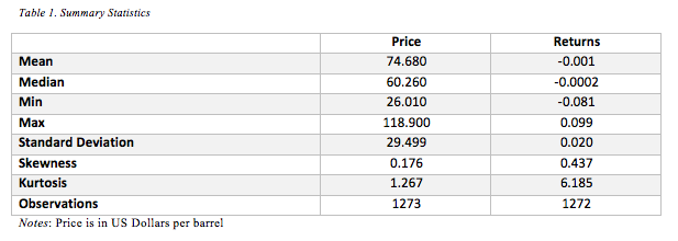
The price appears to exhibit significant changes throughout the period 2012-2017 as evident from the minimum and maximum values. This corresponds to the large drop in oil prices, which occurred in 2014. More importantly, the returns appear to have a substantial number of extreme values as the estimated kurtosis is relatively high. This is consistent with the distributions of returns generally considered to be leptokurtic and have heavier tails compared to the normal distribution (Lucia and Schwartz, 2002; Chung and Wong, 2014).
These observations are further illustrated in Figure 1 showing the behaviour of oil prices and corresponding returns during the 2012-2017 period.
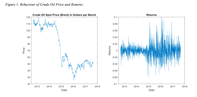
Most notably, a drastic fall in oil prices can be identified in 2014. The presence of two regimes might limit the validity of the models, which do not account for time-varying long-term mean levels. In particular, the parameters estimated for the MRJD model might not reflect the characteristics of pre-2014 and post-2014 periods individually. The discrepancy can also be observed for the plotted returns as the variability seems to increase substantially after the price drop. This may also affect the estimation of jump parameters as extreme returns during the period 2012-2014 would not be identified as jumps due to the higher volatility in the following period.
As the MRJD model extends the GBM approach by potentially accounting for heavier tails, it could be useful to assess the normality of the observed data.
Figure 2 presents the QQ-plot of returns and the histogram with fitted normal distribution.

The observed quantiles show large deviations for more extreme observations compared to normal distribution. Similarly, the fitted normal distribution fails to reproduce the excess kurtosis of the returns. This suggests that it would be more appropriate to estimate the model that accounts for the extreme observations being more likely.
The presence of outliers in the context of the potential presence of two regimes is illustrated in Figure 3.
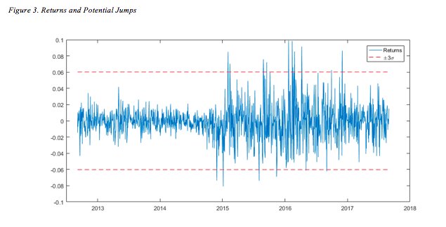
It can be seen that the band of three standard deviations is effectively inflated by the post-2014 outliers compared to the 2012-2014 period. This may lead to potential jumps during a less volatile period being ignored by the recursive filter procedure. In particular, the estimated jump intensity might be too low to reflect sudden changes in returns for both periods.
The independence of observations is assessed by plotting the ACF and PACF of the returns. This is shown in Figure 4.
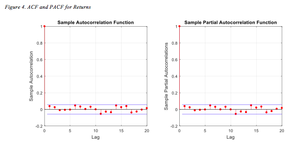
No strong autocorrelation can be seen for the first 20 lags. This suggests that the assumption of independence is appropriate for the return series.
The MRJD model is suggested to capture the potential mean-reverting behaviour of the series. This is investigated more thoroughly by performing ADF and KPSS unit root tests. The results are summarised in Table 2.
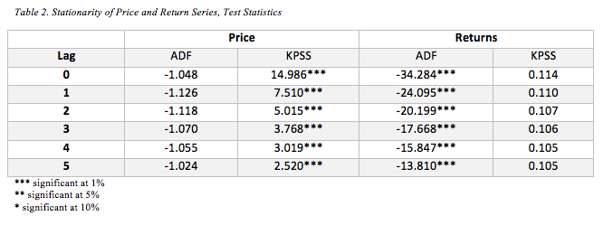
The findings on the price strongly indicate that the series is not stationary. By contrast, all ADF test statistics are significant at the 0.01 level suggesting that the null hypothesis of a unit root should be rejected. This is further supported by the KPSS test. Thus, the returns series can be considered stationary and as such a mean-reversion model would be appropriate.
4.2 MRJD Model Calibration
The estimated MRJD model parameters are presented in Table 3.
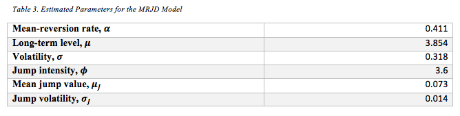
The speed of mean-reversion is relatively low. The value of 0.411 corresponds to the half-life of which equals 1.686 (Clewlow and Strickland, 2000). In other words, it would take the process more than a year to revert half-way to its long-term mean. This could mean that mean-reversion would be less visible for the prices simulated for 126 days. Therefore, it might be expected that the difference between the GBM and MRJD model would be only weakly affected by the mean-reverting behaviour.
The long-term mean of 3.854 represents the mean price of which is equal 47.181. This shows that the model estimation is significantly influenced by the post-2014 years for which lower prices are observed. The value of the jump intensity suggests that, on average, 3.6 jumps occur per year. The relatively low number of jumps can be attributed to the 2012-2014 period being effectively ignored in the recursive filtering procedure. This could have been expected due to the substantially higher volatility in the following years.
The estimation of the mean-reversion parameters relies on the regression of returns on log-prices. The jumps are further explored in this context in Figure 5.
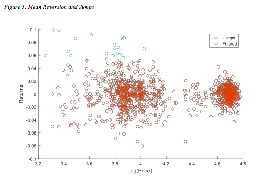
The observations appear to form two major clusters, which represent the potential regime-switching in 2014. This is also visible in all jumps being associated with lower prices, which were only observed during the 2014-2017 years.
Figure 6 shows the identified jumps for both prices and return series.

The jumps seem to occur after substantial drops in price. In particular, several jumps are concentrated at the beginning of 2016. Most notably, the most extreme returns during the 2012-2014 years are still lower compared to the three standard deviations of filtered observations. This suggests that the estimated jump coefficients might not be accurately representing the behaviour of returns during the whole period.
4.3 Simulation
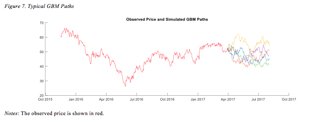
Typical GBM paths simulated for the period after 30 March 2017 are shown in Figure 7.
Mean returns for each simulation show behaviour, which is close to normal. This is illustrated in Figure 8.

The GBM-based returns show no excess kurtosis as the model assumes that the price is log-normally distributed.
Figure 9 presents typical paths simulated by the MRJD approach.
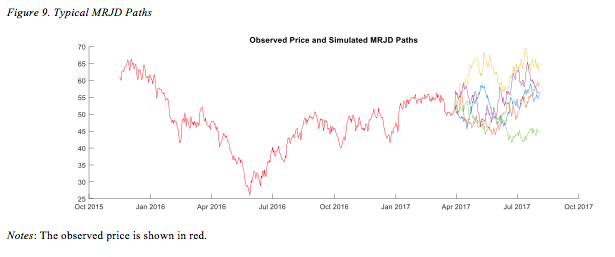
Few observable jumps can be seen, which may be attributed to the low jump intensity compared to the simulation period of 126 days. This is further shown in Figure 10.
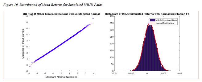
It can be seen that the distribution of returns is still close to normal. In other words, the model could be inaccurately reproducing the observation of heavy tails in the historical returns. This might be explained by the slow mean reversion and low jump intensity estimated for the model.
4.4 Option Pricing and Implied Volatility
The simulated prices are used to determine option premiums for Asian call and put options. The results are summarised in Figure 11 showing the relationship between premium and strike price for options with different expiration dates.
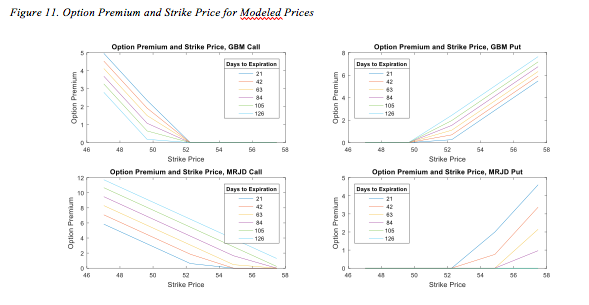
The premium of call options for both models decreases with the strike price as expected. The option loses its intrinsic value as the strike price approaches the average price for the last 21 days of the contract. Likewise, the value of put options increases with the strike price. The call options valued based on the MRJD model appear to have higher premium. This could suggest that the implied volatility would be lower for the GBM model.
The implied volatility surface is shown in Figure 12.
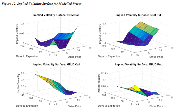
The MRJD-based volatility is lower for the strike values that are closer to the underlying price. The volatility appears to increase as the strike price takes more extreme values. This results in a volatility smile indicating that at-the-money options are associated with the lowest implied volatility. No substantial changes can be observed regarding the time to maturity. It can be seen that the GBM surfaces also exhibit noticeable convexity. This may be attributed to the use of the Black-Scholes pricing formula for arithmetic average options.
The relationship between implied volatility and strike price is further illustrated in Figure 13.
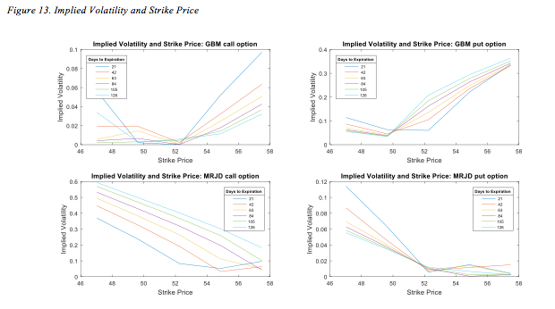
The MRJD-based estimation shows volatility smiles, which are more pronounced for shorter times to maturity. In particular, the options expiring in 21 days are associated with the most noticeable change in implied volatility for both call and put options. At the same time, only small difference can be seen for put options with longer maturities. This can be attributed to the Asian options reducing the impact of time to maturity on the associated uncertainty. Indeed, as the strike price is compared to the average for the last 21 days of the contract, the value of the option would be less prone to the underlying price changes at the time of expiration.
4.5 Discussion
The presence of the volatility smiles for the MRJD model may show that mean reversion and jumps could be sufficient to reproduce the observed behaviour of implied volatility. In other words, this approach could model time-varying volatility due to risk aversion, market imperfections, trading restrictions, and leverage effect (Rubinstein, 1994). This is consistent with the observed implied volatility in the market (Vagnani, 2009; Tankov and Voltchkova, 2009).
Nevertheless, the simulated smiles for the MRJD model are not strongly pronounced. This could be largely attributed to the potential presence of two distinct regimes throughout the period 2012-2017. As a result, both components of the model might have been affected. Firstly, the estimated mean reversion was relatively slow and less observable in the context of 126 trading days. Secondly, the jump intensity could be underestimated as substantial changes during the 2012-2014 period were ignored when compared to the more volatile post-2014 period. This observation highlights the importance of incorporating a regime-switching framework into the model (Weron, 2007; Mitra and Date, 2010).
5. Conclusions
This study focused on the modelling of the behaviour of the Brent crude oil spot prices during the period 2012-2017. Two approaches were used, namely GBM and MRJD models. The GBM model explicitly assumes that the returns are normally distributed, which is in contrast with the observations made on historical data. At the same time, the MRJD model incorporated both mean-reversion and jump components. Nevertheless, the relatively slow speed of mean reversion and low jump intensity resulted in the simulated prices closely following the log-normal distribution. This could be attributed to the presence of two regimes in the underlying series behaviour associated with the 2014 drop in oil prices. The implied volatility surface for the MRJD model suggests that the volatility smile is present with lower volatility corresponding to the at-the-money options.
The study is subject to several limitations. Noticeable errors could be introduced by the discretisation of the underlying stochastic differential equations (Glasserman, 2003). It could be especially relevant for the estimation of Asian options as the variance of the estimated premium would increase with the number of simulated paths (Yang et al., 2009). The study also did not account for the large discrepancy in prices and return volatility between the 2012-2014 and 2014-2017 periods.
Further studies may employ methods for variance reduction to improve the estimation of Asian option premiums (Glasserman, 2003). Alternative approaches can be employed for pricing arithmetic Asian options. This includes binomial trees and Fast Fourier Transform (Hsu and Lyuu, 2011; Fusai and Meucci, 2008). Other methods for jump identification could also be employed. These methods include wavelet filtering and Markov regime-switching model classification (Janczura et al., 2013). Further research could also explore the use of stochastic volatility models (Bormetti et al., 2010; Mitra and Date, 2010). Incorporating regime-switching could result in a more accurate representation of the price behaviour (Mitra and Date, 2010; Weron, 2007).
References
Black, F. and Scholes, M. (1973). The pricing of options and corporate liabilities. The Journal of Political Economy, 81(3), pp.637–654.
Bormetti, G., Cazzola, V., and Delpini, D. (2010). Option pricing under Ornstein-Uhlenbeck stochastic volatility: a linear model. International Journal of Theoretical and Applied Finance, 13(07), pp.1047-1063.
Cartea, A., and Figueroa, M. G. (2005). Pricing in electricity markets: a mean reverting jump diffusion model with seasonality. Applied Mathematical Finance, 12(4), pp.313-335.
Chortareas, G., and Kapetanios, G. (2009). Getting PPP right: identifying mean-reverting real exchange rates in panels. Journal of Banking and Finance, 33(2), pp.390-404.
Chung, S. F., and Wong, H. Y. (2014). Analytical pricing of discrete arithmetic Asian options with mean reversion and jumps. Journal of Banking and Finance, 44, pp.130-140.
Clewlow, L., and Strickland, C. (2000). Energy Derivatives: Pricing and Risk Management. London: Lacima Group.
Dickey, D. A., and Fuller, W. A. (1979). Distribution of the estimators for autoregressive time series with a unit root. Journal of the American Statistical Association, 74(366a), pp.427-431.
Dupire, B. (1997). Pricing and hedging with smiles. Mathematics of Derivative Securities, 1(1), pp.103-111.
EIA. (2017). Petroleum and Other Liquids: Spot Prices. [online] Available at: https://www.eia.gov/dnav/pet/pet_pri_spt_s1_d.htm [Accessed 22 Sep 2017].
Fusai, G., and Meucci, A. (2008). Pricing discretely monitored Asian options under Lévy processes. Journal of Banking and Finance, 32(10), pp.2076-2088.
Geman, H. (2010). Commodities and Commodity Derivatives. Chichester: John Wiley and Sons.
Geman, H., and Roncoroni, A. (2006). Understanding the fine structure of electricity prices. The Journal of Business, 79(3), pp.1225-1261.
Glasserman, P. (2003). Monte Carlo Methods in Financial Engineering. New York: Springer.
Heston, S. L. (1993). A closed-form solution for options with stochastic volatility with applications to bond and currency options. The Review of Financial Studies, 6(2), pp.327-343.
Hsu, W. W., and Lyuu, Y. D. (2011). Efficient pricing of discrete Asian options. Applied Mathematics and Computation, 217(24), pp.9875-9894.
Jablonska, M. (2011). The multiple-mean-reversion jump-diffusion model for Nordic electricity spot prices. The Journal of Energy Markets, 4(2), pp.3-25.
Janczura, J., Trück, S., Weron, R., and Wolff, R. C. (2013). Identifying spikes and seasonal components in electricity spot price data: A guide to robust modeling. Energy Economics, 38, pp.96-110.
Kwiatkowski, D., Phillips, P. C., Schmidt, P., and Shin, Y. (1992). Testing the null hypothesis of stationarity against the alternative of a unit root: How sure are we that economic time series have a unit root? Journal of Econometrics, 54(1-3), pp.159-178.
Lucia, J. J., and Schwartz, E. S. (2002). Electricity prices and power derivatives: Evidence from the Nordic power exchange. Review of Derivatives Research, 5(1), pp.5-50.
Merton, R. C. (1976). Option pricing when underlying stock returns are discontinuous. Journal of financial economics, 3(1-2), pp.125-144.
Mitra, S. (2011). A review of volatility and option pricing. International Journal of Financial Markets and Derivatives, 2(3), pp.149-179.
Mitra, S., and Date, P. (2010). Regime switching volatility calibration by the Baum–Welch method. Journal of Computational and Applied Mathematics, 234(12), pp.3243-3260.
Rubinstein, M. (1994). Implied binomial trees. The Journal of Finance, 49(3), pp.771-818.
Schwartz, E., and Smith, J. E. (2000). Short-term variations and long-term dynamics in commodity prices. Management Science, 46(7), pp.893-911.
Tankov, P., and Voltchkova, E. (2009). Jump-diffusion models: a practitioner’s guide. Banque et Marchés, 99(1), pp.24-47.
Vagnani, G. (2009). The Black–Scholes model as a determinant of the implied volatility smile: A simulation study. Journal of Economic Behavior and Organization, 72(1), pp.103-118.
")