Written by Carl R.
Security holdings become riskier when stock prices fluctuate. Such fluctuations are commonly regarded as volatility, whereas, minor ones tend to be considered market noise (i.e. the shifting positions of investors on inter-day trading). Thus, as investors move to enhance their positions, a number of variables are taken into account, such as macroeconomic conditions, accounting statements and industry trends. Option valuation also takes these variables into account by using the present value of the stock price as a benchmark on which hedges will be formed. The major variables used to derive an option’s price are current stock price, intrinsic value, time to expiration, and volatility (Bodie et al., 2009). Therefore, options can best be described as ways in which investors can take advantage of superior information to hedge against their current stock positions.
The value of the option is derived from the current stock price, thus when a profitable position is determined the option is called “in the money” whereas a position in which profit is zero is considered “out of the money” (Ward, 2004). Simple notation below describes this relationship:

In option trading, profit is achieved when an investor sells a share between the strike price (the price when an investor can sell) and the stock price. Different option positions, therefore, garner different names. Table 1, below, show the two fundamental options upon which all other financial instruments are formed:
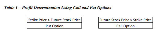
The above relationships indicate the basic positions an investor could have on a stock’s future value: outperform expectations (call option) or underperform expectations (put option). Thus, profit is achieved the greater the difference between the strike price and stock price at the call time, allowing the investor to take advantage of their position.
As the product’s future price clarifies, the stock option becomes less volatile. One reason for this outcome is related to the idea that option prices become firm as uncertainty (time) is removed from the equation; the option value will be larger the further away from the call date. Using the martingale explanation given by McCauley et al. (2007), the option price becomes fixed as the call date manifests. Geometrically, this outcome is represented as a high peak centered on the given price at the current time. Stocks, therefore, with little non-time related volatility have options with firm prices beyond the call time.
While non-time related volatility at the call time marginally affects the option price, the moments leading up to the call time could exhibit high volatility because of factors such as industry position, poor performance and historical trends. Industry position and poor performance are based on the fundamental approach to investing, which bases a firm’s position vis-à-vis other firms in the industry. Volatility measured using this approach is considered implied volatility; volatility measured along historical trends is regarded as historical volatility. Most investors use a weighted combination to create a specific volatility measure (Chen et al., 2018).
The different measures of riskiness are used to develop specific outcomes; specifically, the exact probabilities determine the upper and lower bounds of a call period. The difference between the predicted upper bound and the current stock price leads to the payback quantity, whereas the present value of the lower bound over upper bound ratio multiplied by the lower bound stock price creates the amount necessary to borrow in order to achieve the same value as the profit generated from upper bound estimate. The value of the stock price times the ratio minus the loan thus generates the option price (Hull, 2017).
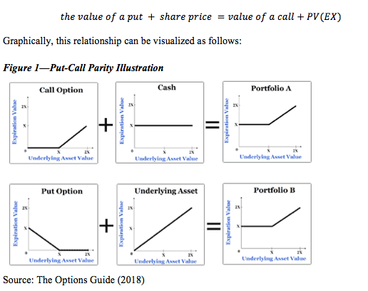
The ratio of the complicated process is commonly regarded as the options delta which takes the range of the possible payoffs over the range of the possible prices. When the options delta is multiplied by the stock price then subtracted by the loan size, the option price is generated. The option price for a put and call option are connected by the relationship called the put-call parity defined below:
The binomial method for option valuation is useful when analyzing European options because options cannot be called in beforehand (Hull, 2017). As more options are added to the scenario the spread becomes increasingly continuous, such that the options tree evolves into what is known as the binomial method for valuing options. Equation 1, below, highlights the relationship between the upper and lower bound (Brealey and Meyers 2003):

Such that e is the base of natural logs, sigma is the standard deviation of the company’s stock returns and h is the fraction of the time interval.
While the binomial method for valuation of options is useful when the risk similar throughout a time period, the Monte Carlo method is more useful, when sources of uncertainty can change throughout the period and when uncertainty arises from multiple sources. By running thousands of scenarios, this method generates the most likely outcomes given the specified parameters. The amount of time necessary to properly set up the scenario, though, makes this method impractical; for most purposes, the Monte Carlo method is used as a last resort, only utilized for the most complex scenarios (Sun and Xu, 2018).
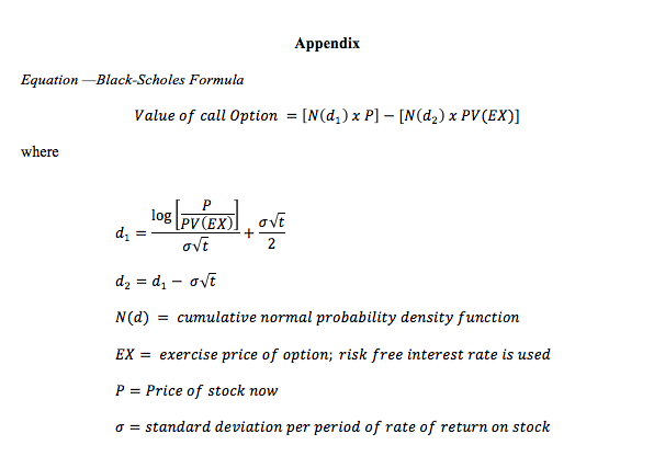
The Black-Scholes Option Pricing Formula, regarded as the backbone of the options market, is an equation by which many options are priced. The complete equation, listed in Appendix, examines the relationship between the probabilities of the forward price and the strike price; however, forward prices have little value in measuring current prices and the reversion back to the present value is necessary. The Black Scholes equation converts the expanding factor of into a decaying factor and multiplies it throughout the equation such that the forward price is reverted to the spot price and the strike price is measured in present value terms (Brealey and Meyers 2003).
The above relationship fails to account for the probability of the terms, thus when accounting for the normal distribution (N(d)), the model assumes only one true probability: the probability of the strike price. The spot price fluctuates with the various components of the model, and thus so does the probability. However, the Greeks (derivatives found in the model) are used primarily to help bring additional certainty to the investor.
Perhaps the most important Greek is delta (which observes the rate of change between the call premium and the spot price. As this is a rate of change the value typically is between 0-1, such that a value .10 indicates the option moves 10% as fast as the actual stock. The lower the delta the more stable the option, hence is a safer investment. Larger stocks, in mature firms have the tendency to have lower deltas, while smaller firms usually retain higher ones. Commonly though, delta is unstable and fluctuates between faster and slower points. The rate at which these fluctuations happen is considered gamma (Shafi et al., 2018).
While delta is often referred to as the most important Greek, gamma is widely regarded as the second most important one, mainly because it observes delta’s rate of change. The concept is regarded as the ability of the option to change from relatively safe to relatively risky. Thus the equation is often represented as the second derivative of delta:
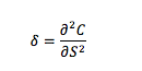
When gamma is high, delta can change rapidly, which could bring excessive risk to the investor looking to hedge with an option. As delta inevitably becomes unstable, gamma is useful for finding the point at which delta begins to increase rapidly. The other Greeks help perform similar tasks as well (Hull, 2017; Shafi et al., 2018).
The effect of time is one measure which many analysts take into account when purchasing an option. The Greek symbol theta ( finds the rate at which time decays the option. Thus, when the option decays at a relatively quick pace, the option is deemed to be worth less than that which does not. Theta is usually measured on a daily basis as to give a benchmark for the analysis. Shorter time periods, such as seconds and hours are impractical formal analysis. Time exposure’s basic component shows the best point for selling an option (Khaliq et al., 2008).
Selling an option, as discussed earlier, can fluctuate greatly if the volatility is high. The Greek used to measure volatility is vega (also called kappa) (. This measure greatly influences the price of the option by illustrating the underlying risk associated with it. Thus, when the call premium exhibits excessive volatility, vega will increase. In essence, the structure of the options market centers on the idea of volatility, because it is the one unknown determined in the equation. Therefore, exposing against excessive volatility is difficult for option’s traders to accomplish. Tools such as SV, ARCH and GARCH models try to predict future volatility, but even so, these tools are modestly effective and incapable of predicting the dramatic effects of crises (Papantonis, 2016; Wang et al., 2017).
Each Greek is used to discover a particular risk in the model; specifically, gamma and delta monitor spot price risk exposure, theta monitors time risk exposure, and vega observes volatility exposure. Thus, these factors help decide where excessive risk is clustering. The smaller Greek, rho (, monitors interest rate risk, and is usually a small problem for larger companies. This risk could be a major factor in smaller firms (Hull, 2017).
Conceptually neutralizing risk is largely doing the opposite of the option the investor is purchasing. For example, if an investor bought 300 call options which can call 15,000 shares, when the option delta of the call option is .20, the exposure would equal [15,000 x .20 = 3,000]. This equation signifies the exposure of the investor would be like owning 3,000 shares of the stock; in order to neutralize the hedge, the investor should sell short 3,000 shares in order to reduce the exposure back to zero. However, as delta is always changing, the required shares to remain neutralized would fluctuate up and down, thus the investor would have to participate in what is commonly referred to as dynamic hedging. A practical exercise discussing the relationship between the put and call European options should further explain the subtle relationship of put and call options.
References
Brealey, R.A., and Meyers, S.C. (2003). Finance: McGraw-Hill, Primis online: text, Principles of Corporate Finance, Seventh edition. Boston: McGraw-Hill/Irwin.
Bodie, Z., Kane, A. and Marcus, A. (2009). Investments. New York: Irwin/McGraw Hill.
Chen, Y., Han, Q. and Niu, L., 2018. Forecasting the term structure of option implied volatility: The power of an adaptive method. Journal of Empirical Finance.49, pp.157-177.
Hull, J. (2017) Options, Futures and Other Derivatives, London: Pearson.
Khaliq, A.Q., Voss, D.A. and Kazmi, K., (2008). Adaptive θ-methods for pricing American options. Journal of Computational and Applied Mathematics, 222(1), pp.210-227.
McCauley, J.L., Gunaratne, G.H. and Bassler, K.E., (2007). Martingale option pricing. Physica A: Statistical Mechanics and its Applications, 380, pp.351-356.
Papantonis, I., (2016). Volatility risk premium implications of GARCH option pricing models. Economic Modelling, 58, pp.104-115.
Samuelson, P. (1965) Proof that Properly Anticipated Prices Fluctuate Randomly. Industrial Management Review, 6 (2), p.41-49.
Shafi, K., Latif, N., Shad, S.A., Idrees, Z. and Gulzar, S., (2018). Estimating option greeks under the stochastic volatility using simulation. Physica A: Statistical Mechanics and its Applications, 503, pp.1288-1296.
Sun, Y. and Xu, C., (2018). A hybrid Monte Carlo acceleration method of pricing basket options based on splitting. Journal of Computational and Applied Mathematics, 342, pp.292-304.
The Options Guide (2018) Understanding Put-Call Parity, Available at: http://www.theoptionsguide.com/understanding-put-call-parity.aspx [Accessed on 6 November 2018].
Wang, G., Wang, X. and Zhou, K., (2017). Pricing vulnerable options with stochastic volatility. Physica A: Statistical Mechanics and its Applications, 485, pp.91-103.
Ward, R. W. (2004). Options and options trading a simplified course that takes you from coin tosses to Black-Scholes. New York: McGraw-Hill.
Appendix
")